[ad_1]
In this study, we utilized the Traditional Indian Art Painting Art Dataset (TIAPD) to evaluate our proposed methodology, which comprises a diverse collection of traditional Indian art images. Our methodology includes automatic learning-based feature extraction techniques, with a CNN model employed for the retrieval of images. Various similarity measures and performance metrics are then used for the evaluation to ensure validation of the proposed methodology.
Dataset description
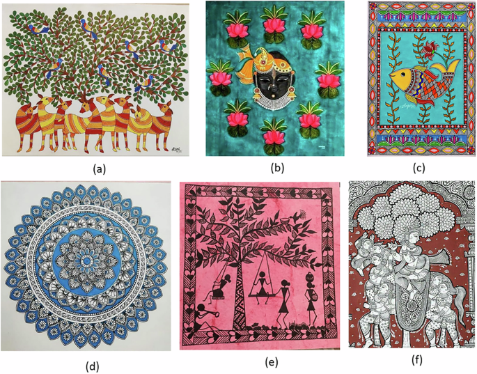
The images of the TIAPD used in this study were collected from Pinterest33, a popular social networking site with strong visual content. Different images from various art forms like Gond, Pichwai, Madhubani, Mandala, Warli, and Kalamkari are included in the dataset as shown in Fig. 1. Each art form is represented by images that are visually distinct and characterize the respective art form. Identifying and classifying images according to their art form is one of the main purposes of the dataset, which is meant to be used for image retrieval applications. The dataset is distinctive because it contains a wide variety of art forms and a substantial number of images, which makes it an excellent resource for developers and scholars studying computer vision and image processing. The dataset contains 600 images, with 100 images belonging to each category.

a Gond painting, b Pichwai painting, c Madhubani Painting, d Mandala Painting, e Warli Painting, and e Kalamkari painting.
Furthermore, for the validation of the results of the proposed methods, simulations are also conducted on various conventional datasets, in addition to the TIAPD dataset. These datasets include:
-
1.
Wang-A: This dataset has been widely used for image retrieval and classification tasks34. It comprises 1000 images that belong to 10 different categories.
-
2.
OT Scene: This dataset comprises 2688 images of outdoor locations divided into 8 different categories35.
-
3.
Wang 10k: There are 10,000 images in this database distributed into 100 classes36.
-
4.
Caltech 256: This dataset has been commonly used for object recognition and image classification37. It comprises 30,607 images categorized into 257 object categories.
-
5.
Corel-1K: This dataset comprises 1000 images of 10 distinct classes. This database has been commonly employed in image retrieval tasks38.
By conducting trials on these standardized datasets, the study ensures that the proposed techniques are not only efficient for the TIAPD dataset but also have good generalizability to other types of image data.
Proposed methodology
The main modules of the research methodology are reading of images, resizing of images, extraction of features, reduction of features, and retrieval of images from the TIAPD. The flow chart of the methodology is shown in Fig. 2. In this methodology, initially TIAPD dataset is used as input. Each image of this dataset is resized to 224 × 224 pixels to ensure uniformity of all images. After resizing, feature extraction is performed using two CNN models: ResNet50V2 and EfficientNetB0. These pre-trained networks are selected for their ability to capture both high-level and low-level features from images. Both these features are important for the retrieval of images in an accurate way because they contain information about important characteristics of images. High-level features include information about the shape of objects, patterns, etc., while low-level features contain information about colors, edges, and textures of the image.

Block diagram of proposed methodology
ResNet50V239, as shown in Fig. 3, is a version of the Residual Networks (ResNet) architecture that helps mitigate the vanishing gradient problem and allows the network to learn complex features effectively. On the other hand, EfficientNetB040, as shown in Fig. 4, uses a compound scaling method, leading to high efficiency with fewer parameters.

Architecture of ResNet50V2

Architecture of EfficientNetB0
After the extraction of features from both models, all these features are concatenated to improve the robustness of the feature set, which provides a more detailed understanding of the images. The fusion of both these models is important to extract all features of the image for performing the image retrieval process in an efficient way. After the concatenation of features, the RFE technique is applied to all features for the reduction of feature space and computational complexity of the algorithm. This RFE technique reduces the feature space by preserving the most significant features.
This similar process, which includes resizing of the image, extraction of features using both pre-trained models, concatenations of features, and reduction of features using RFE, is applied to the query image also. Features extracted from all database images and query images are important to check the similarity measurement between them. To accomplish the task of similarity measurement, different distance metrics like Euclidean, Cosine Similarity, Manhattan, Minkowski, Hamming, and Jaccard are used, and distances computed by different distance methods are sorted in ascending order to get the most relevant images at the top. The retrieved images are ranked based on their similarity to the query image. In the end, the efficacy of the system is assessed using different evaluation metrics like mean average precision, recall, and F1-score. Algorithm 1 presents the pseudo-code of the proposed methodology.
Algorithm 1
Content-Based Image Retrieval of traditional Indian paintings
Input:
• Database of images: D = {I1, I2,…. IN}
• Query Image Q
Output:
• Top k most similar images to the query Q
1. Initialize pre-trained models:
• Load EfficientNetB0 and ResNet50V2 models without the final classification layers
2. Read and Resize Image:
• Define a function read_and_resize_image (image_path) to:
• Read the image from image_path
• Resize the image to 224 × 224 pixels
• Return the resized image
3. Extract features:
• Define a function extract_features (resized image, model) to:
• Pass the resized image through the model.
• Extract features from the intermediate layers.
• Return the feature vector.
4. Extract and concatenate features for Database images:
• Initialize an empty list to store features for all database images.
• For each Ii in D:
• Read and resize Ii using read_and_resize_image.
• Extract features \({f}_{i}^{{M}_{1}}\) from EfficientNetB0 and \({f}_{i}^{{M}_{2}}\) from ResNet50V2 using extract_features
• Concatenate the features:
$${f}_{i}=[{f}_{i}^{{M}_{1}\,}{{\rm{||}}f}_{i}^{{M}_{2}}]$$
• Store \({f}_{i}\) in the list.
5. Extract and Concatenate features for query image
• Read and resize Q using read_and_resize_image
• Extract features \({f}_{Q}^{{M}_{1}}\) and \({f}_{Q}^{{M}_{2}}\).
• Concatenate the features:
$${f}_{Q}=[{f}_{Q}^{{M}_{1}\,}{{\rm{||}}f}_{Q}^{{M}_{2}}]$$
6. Dimensionality reduction using RFE
• Define a function apply_rfe(features,estimator) to:
• Apply Recursive Feature Elimination (RFE)
• Select the optimal subset of features
• Return the reduced feature set.
• Apply RFE to both \({f}_{Q}\) and \({f}_{i}\)
7. Compute distance scores
• Initialize an empty list for distance scores.
• For each \({f}_{i}^{{Reduced}}\) in the database:
• Compute the Euclidean distance between \({f}_{i}^{{Reduced}}\) and \({f}_{Q}^{{Reduced}}\) .
$$d=\,\sqrt{\mathop{\sum }\limits_{j=1}^{n}{({f}_{Q,j}^{{Reduced}}-{f}_{i,j}^{{Reduced}})}^{2}}$$
• Store d in the list.
8. Rank Database Images Based on Distance Scores:
• Sort the database images in ascending order of distance scores.
9. Output the Top k most Similar Images:
• Retrieve and display the top k images with the lowest distance scores.
Distance metrics
The distance metrics are used to find the most relevant images related to the query image. To find the similarity between the images, the features of both the query image and the database images are represented as feature vectors. Different distance metrics used to compute distances using feature vectors for image retrieval are given below:
-
a.
Euclidean Distance: It computes the straight-line distance between two feature vectors. It can be calculated using Eq. (1).
$$d\left(q,{x}_{i}\right)=\sqrt{\mathop{\sum }\limits_{j=1}^{n}{({q}_{j}-{x}_{{ij}})}^{2}}$$
(1)
Here, \(d\left(q,{x}_{i}\right)\) represents the distance computed between query image and the dataset retrieved image, n represents the number of features in feature vectors, q is the feature vector of the query image, which is represented by [q1, q2, q3, …., qn] and \({x}_{{ij}}\) is the feature vector of the retrieved images. Here, xi, which is the feature vector of the ith retrieved images, is represented as [xi1, xi2, xi3, …., xin]
-
b.
Cosine Similarity: The formula used to compute cosine similarity is given by Eq. (2). It is used to measure the cosine of the angle between two image feature vectors.
$${\rm{cosine}}\; {\rm{similarity}}\left(q,{x}_{i}\right)=\frac{q.{x}_{i}}{{||q||\,||}{x}_{i}{||}}$$
(2)
-
c.
Manhattan Distance: The formula used to measure the Manhattan distance metric is given by Eq. (3). It calculates the dissimilarity between two feature vectors by summing the absolute differences of their coordinates.
$$d\left(q,{x}_{i}\right)=\mathop{\sum }\limits_{j=1}^{n}\left|{q}_{j}-{x}_{{ij}}\right|$$
(3)
-
d.
Minkowski Distance: This similarity measure is a generalization of Euclidean and Manhattan distance. The formula of Manhattan distance is shown by Eq. (4).
$$d\left(q,{x}_{i}\right)={\left(\mathop{\sum }\limits_{j=1}^{n}{\left|{q}_{j}-{x}_{{ij}}\right|}^{p}\right)}^{\frac{1}{p}}$$
(4)
where p defines the order of the distance metric.
-
e.
Hamming Distance: This distance is applicable for feature vectors that are binary in nature and is given by Eq. (5). To calculate the similarity between two feature vectors, it determines the bit positions where the two binary strings differ.
$$d\left(q,{x}_{i}\right)=\mathop{\sum }\limits_{j=1}^{n}({q}_{j}\ne {x}_{{ij}})$$
(5)
-
f.
Jaccard Similarity: It measures the similarity of two sets by taking the ratio of their intersection with their union. It is given by Eq. (6).
$${Jaccard\; similarity}\left(q,{x}_{i}\right)=\frac{\left|Q\cap {X}_{i}\right|}{\left|Q\cup {X}_{i}\right|}$$
(6)
where Q and Xi are the sets of indices where q and xi have non-zero values.
Evaluation of performance metrics
To check the efficacy of the proposed CBIR system, precision, recall, and F1-score fundamental metrics are used. Precision represents the accuracy of the system by computing the relevancy of images against retrieved images for the query image. The formula used to calculate precision is represented by Eq. (7). Recall represents the robustness of the system by identifying all the relevant images of the dataset. The formula used to evaluate recall is shown by Eq. (8). The F1-score is a measure of a model’s accuracy, which provides a balance between the precision and recall. The formula used to compute the F1-score is given by Eq. (9). To compute these metrics, the model is applied to the query image to get the relevant images from the dataset. After visualizing the results, the number of relevant images are checked, and then performance metrics are evaluated based on the quantitative analysis of images.
$${{Precision}\,({Pre}})=\frac{{{Number\; of\; relevant\; images\; retrieved}}\,}{{{Total\; number\; of\; images\; reterieved}}}$$
(7)
$${{Recall}\,({Rec}})=\frac{{{Number\; of\; relevant\; images\; retrieved}}\,}{{{Total\; number\; of\; relevant\; images\; in\; the\; dataset}}}$$
(8)
$$F1\,{{Score}}(F1)=\,\frac{2* {{Pre}}* {{Rec}}}{{{Pre}}+{{Rec}}}$$
(9)
In the proposed work, precision, recall, and F1-score are computed for each query image. So, to show the effectiveness of the entire system, average of both these metrices has been taken for each category of the TIAPD dataset. Where Eq. (10), Eq. (11), and Eq. (12) representing the average precision, average recall, and average F1-score, respectively.
$${{Average\; Precision}}\,\left({{APre}}\right)=\,\frac{1}{C}\mathop{\sum }\limits_{n=1}^{C}{{Pre}}(n)$$
(10)
Here, C represents the number of query images for each category.
$${{Average\; Recall}}\,({{ARec}})=\frac{1}{C}\mathop{\sum }\limits_{n=1}^{C}{{Rec}}(n)$$
(11)
$${{Average}}\,F1\,{{Score}}({{AF}}1)=\frac{1}{C}\mathop{\sum }\limits_{n=1}^{C}F1(n)$$
(12)
To represent the precision, recall, and F1-score of the proposed CBIR system, mean average precision, mean average recall, and mean average F1-score are computed for the complete dataset as represented by Eq. (13), Eq. (14), and Eq. (15), respectively.
$${{Mean\; Average\; Precision}}\,\left({{mAPre}}\right)=\,\frac{1}{N}\mathop{\sum }\limits_{n=1}^{N}{{APre}}(n)$$
(13)
$${{Mean\; Average\; Precision}}\,\left({{mARec}}\right)=\,\frac{1}{N}\mathop{\sum }\limits_{n=1}^{N}{{ARec}}(n)$$
(14)
$${{Mean\; Average}}\,F1\,{{Score}}\left({\rm{mAF}}1\right)=\,\frac{1}{N}\mathop{\sum }\limits_{n=1}^{N}{{AF}}1(n)$$
(15)
Here, N represents the number of categories of the TIAPD dataset.
[ad_2]
Source link